Pygal: Elegant and Interactive Data Visualization in Python

Visualizing Data with Pygal: A Beginner-Friendly Guide to Interactive Graphs in Python

Introduction:

Pygal is an open source user friendly Python Library that enables highly customizable SVG(Scalable Vector Graphics) charts. With it, you can generate charts that are perfect for web applications, reports and presentations. It integrates well with frameworks like FLash and Django and its output visualization is quick and elegant.

Installation and Setup

Use package manager pip

! pip install pygal

Collecting pygal
  Downloading pygal-3.0.5-py3-none-any.whl.metadata (3.5 kB)
Requirement already satisfied: importlib-metadata in /usr/local/lib/python3.11/dist-packages (from pygal) (8.6.1)
Requirement already satisfied: zipp>=3.20 in /usr/local/lib/python3.11/dist-packages (from importlib-metadata->pygal) (3.21.0)
Downloading pygal-3.0.5-py3-none-any.whl (129 kB)
   ━━━━━━━━━━━━━━━━━━━━━━━━━━━━━━━━━━━━━━━━ 129.5/129.5 kB 1.2 MB/s eta 0:00:00
Installing collected packages: pygal
Successfully installed pygal-3.0.5

import into the script
import pygal

If you are in jupyter notebook:

! pip install ipython

! pip install cairosvg

Then, configure your notebook:

from IPython.display import SVG, display
def show_svg(svg):
    display(SVG(svg.render()))

Key Features & Explanation:

Customizable Styles:

Modify colors, labels, and tooltips to suit your needs.

Browser-Friendly:

SVG charts can be easily embedded in web pages.

Export Options:

Export charts as PNG, PDF, or other formats using additional libraries.

Wide Range of Chart Types: Supports bar: Pygal’s Bar chart allows you to plot data for different categories and add multiple series.

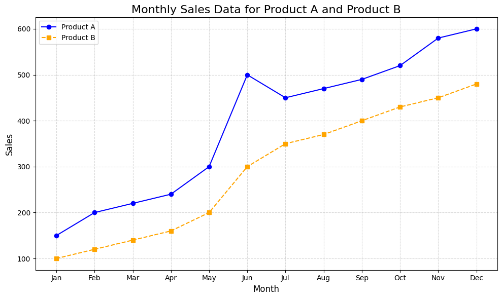
Line:

Line charts are used to display information as a series of data points connected by straight lines.

Using matplotlib:

import matplotlib.pyplot as plt

months = ['Jan', 'Feb', 'Mar', 'Apr', 'May', 'Jun', 'Jul', 'Aug', 'Sep', 'Oct', 'Nov', 'Dec']
product_a = [150, 200, 220, 240, 300, 500, 450, 470, 490, 520, 580, 600]
product_b = [100, 120, 140, 160, 200, 300, 350, 370, 400, 430, 450, 480]

plt.figure(figsize=(10, 6))
plt.plot(months, product_a, label='Product A', marker='o', linestyle='-', color='blue')
plt.plot(months, product_b, label='Product B', marker='s', linestyle='--', color='orange')

plt.title('Monthly Sales Data for Product A and Product B', fontsize=16)
plt.xlabel('Month', fontsize=12)
plt.ylabel('Sales', fontsize=12)
plt.legend()
plt.grid(True, linestyle='--', alpha=0.5)

plt.tight_layout()
plt.show()

Using pygal:

import pygal

line_chart = pygal.Line()
line_chart.title = 'Monthly Sales Data (2024)'
line_chart.x_labels = map(str, range(1, 13))
line_chart.add('Product A', [150, 200, 220, 240, 300, 500, 450, 470, 490, 520, 580, 600])
line_chart.add('Product B', [100, 120, 140, 160, 200, 300, 350, 370, 400, 430, 450, 480])
line_chart.render_to_file('line_chart.svg')

display(SVG('line_chart.svg'))

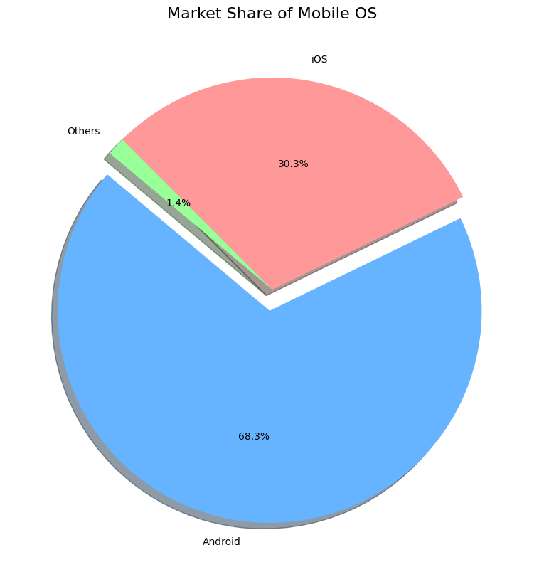
pie:

They’re useful for displaying how different parts make up a total.

Using Matplotlib:

import matplotlib.pyplot as plt

labels = ['Android', 'iOS', 'Others']
sizes = [68.3, 30.3, 1.4]
colors = ['#66b3ff', '#ff9999', '#99ff99']
explode = (0.1, 0, 0)

plt.figure(figsize=(8, 8))
plt.pie(sizes, labels=labels, colors=colors, autopct='%1.1f%%', startangle=140, explode=explode, shadow=True)

plt.title('Market Share of Mobile OS', fontsize=16)

plt.tight_layout()
plt.show()

Using Pygal:

import pygal

pie_chart = pygal.Pie()
pie_chart.title = 'Market Share of Mobile OS'

pie_chart.add('Android', 68.3)
pie_chart.add('iOS', 30.3)
pie_chart.add('Others', 1.4)

pie_chart.render_to_file('pie_chart.svg')

display(SVG('pie_chart.svg'))

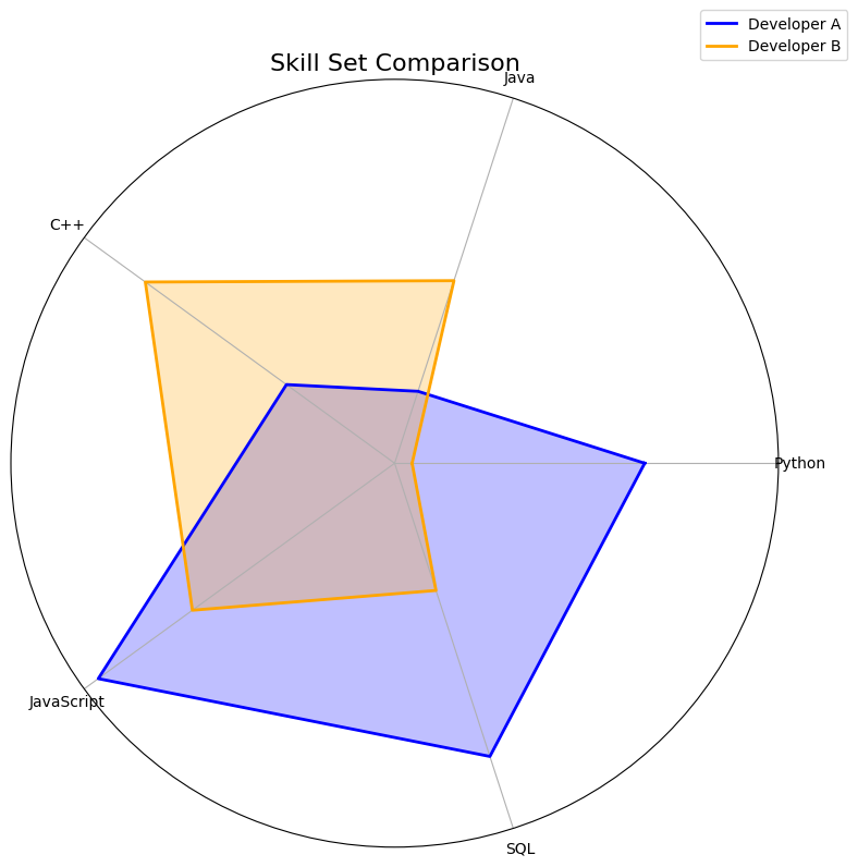
Radar:

Radar charts display multivariate data on axes starting from the same point. They are good for comparing multiple variables.

Using Matplotlib:

import matplotlib.pyplot as plt
import numpy as np

labels = ['Python', 'Java', 'C++', 'JavaScript', 'SQL']
developer_a = [80, 65, 70, 90, 85]
developer_b = [60, 75, 85, 80, 70]

angles = np.linspace(0, 2 * np.pi, len(labels), endpoint=False).tolist()
developer_a += developer_a[:1]
developer_b += developer_b[:1]
angles += angles[:1]

fig, ax = plt.subplots(figsize=(8, 8), subplot_kw=dict(polar=True))

ax.plot(angles, developer_a, label='Developer A', color='blue', linewidth=2)
ax.fill(angles, developer_a, color='blue', alpha=0.25)

ax.plot(angles, developer_b, label='Developer B', color='orange', linewidth=2)
ax.fill(angles, developer_b, color='orange', alpha=0.25)

ax.set_yticks([])
ax.set_xticks(angles[:-1])
ax.set_xticklabels(labels)

plt.title('Skill Set Comparison', fontsize=16)
ax.legend(loc='upper right', bbox_to_anchor=(1.1, 1.1))

plt.tight_layout()
plt.show()

Using Pygal:

import pygal

radar_chart = pygal.Radar()
radar_chart.title = 'Skill Set Comparison'

radar_chart.x_labels = ['Python', 'Java', 'C++', 'JavaScript', 'SQL']

radar_chart.add('Developer A', [80, 65, 70, 90, 85])
radar_chart.add('Developer B', [60, 75, 85, 80, 70])
radar_chart.render_to_file('radar_chart.svg')

display(SVG('radar_chart.svg'))

Exporting and Embedding Charts in Pygal

One of Pygal’s strengths is that it can export charts as SVG files, which stay clear and sharp at any size. Example:

import pygal

bar_chart = pygal.Bar()
bar_chart.add('Cats', [1, 2, 3])
svg_data = bar_chart.render()

with open('chart.html', 'w') as file:
    file.write(f'<html><body>{svg_data}</body></html>')

Interactive SVG Output:

Charts are rendered as SVGs, making them scalable and interactive.

Using Matplotlib:

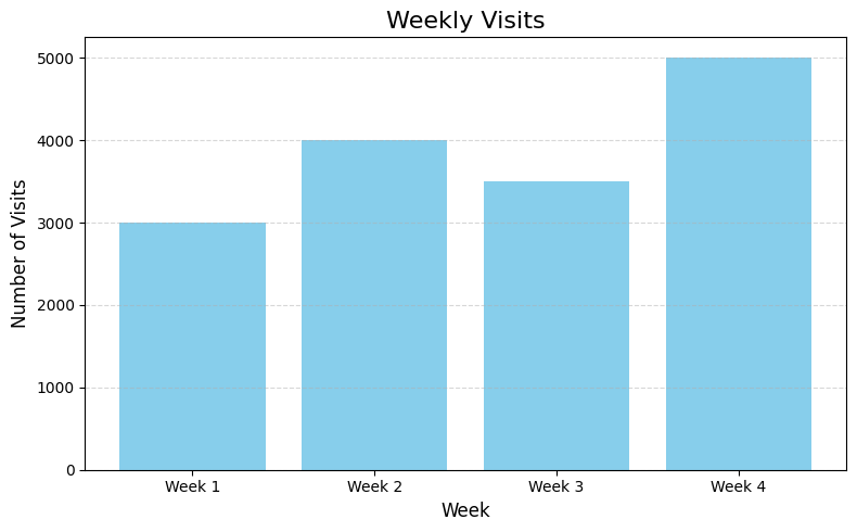
import matplotlib.pyplot as plt

weeks = ['Week 1', 'Week 2', 'Week 3', 'Week 4']
visits = [3000, 4000, 3500, 5000]

plt.figure(figsize=(8, 5))
plt.bar(weeks, visits, color='skyblue')

plt.title('Weekly Visits', fontsize=16)
plt.xlabel('Week', fontsize=12)
plt.ylabel('Number of Visits', fontsize=12)
plt.grid(axis='y', linestyle='--', alpha=0.5)

plt.tight_layout()
plt.show()

Using Pygal:

bar_chart = pygal.Bar()
bar_chart.title = 'Website Visits per Week'
bar_chart.x_labels = ['Week 1', 'Week 2', 'Week 3', 'Week 4']
bar_chart.add('Visits', [3000, 4000, 3500, 5000])
bar_chart.render_to_file('bar_chart.svg')

display(SVG('bar_chart.svg'))

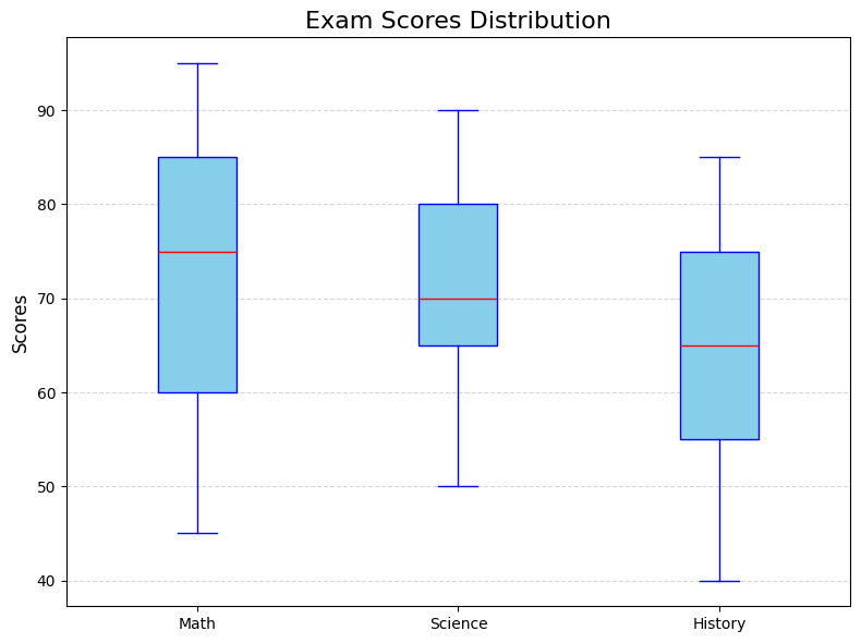
Box plots:

Box plots are used to display the distribution of data based on five summary statistics: minimum, first quartile, median, third quartile, and maximum. and more.

Using Matplotlib:

import matplotlib.pyplot as plt

scores = {
    'Math': [45, 60, 75, 85, 95],
    'Science': [50, 65, 70, 80, 90],
    'History': [40, 55, 65, 75, 85]
}

data = [scores['Math'], scores['Science'], scores['History']]
labels = list(scores.keys())

plt.figure(figsize=(8, 6))
plt.boxplot(data, labels=labels, patch_artist=True,
            boxprops=dict(facecolor='skyblue', color='blue'),
            medianprops=dict(color='red'),
            whiskerprops=dict(color='blue'),
            capprops=dict(color='blue'))

plt.title('Exam Scores Distribution', fontsize=16)
plt.ylabel('Scores', fontsize=12)
plt.grid(axis='y', linestyle='--', alpha=0.5)

plt.tight_layout()
plt.show()

MatplotlibDeprecationWarning: The 'labels' parameter of boxplot() has been renamed 'tick_labels' since Matplotlib 3.9; support for the old name will be dropped in 3.11.
  plt.boxplot(data, labels=labels, patch_artist=True,

Using Pygal:

import pygal

box_plot = pygal.Box()
box_plot.title = 'Exam Scores Distribution'

box_plot.add('Math', [45, 60, 75, 85, 95])
box_plot.add('Science', [50, 65, 70, 80, 90])
box_plot.add('History', [40, 55, 65, 75, 85])

box_plot.render_to_file('box_plot.svg')

display(SVG('box_plot.svg'))

Creating Dynamic Charts with Pygal

One of Pygal’s key strengths is its ability to create dynamic charts by integrating with Python’s data structures. This enables charts to update automatically in response to real-time or changing datasets, making Pygal a great option for dashboards, reports, and web applications that need continuously updated data. example:

import pygal

data = {'Cats': [1, 2, 3], 'Dogs': [4, 5, 6]}
bar_chart = pygal.Bar()
for key, values in data.items():
    bar_chart.add(key, values)
bar_chart.render_to_file('bar_chart.svg')

display(SVG('bar_chart.svg'))

Use cases:

Web Dashboards: Embedding interactive charts for user analytics.

Data Reports: Creating professional-looking charts for business insights.

Educational Content: Visualizing mathematical functions and data sets for teaching.

Scientific Research: Plotting experimental results interactively

Conclusion:

Pygal is an excellent choice for Python developers seeking quick, interactive, and visually appealing data visualizations. Its SVG output ensures charts look sharp at any size, making them perfect for both web and print. The simplicity of its API combined with a variety of chart types allows you to present data in the most effective and engaging way.

REFERENCES and FURTHER READINGS

Official Documentation:
https://www.pygal.org/en/3.0.0/documentation/index.html

Other references:
1) https://www.analyticsvidhya.com/blog/2022/04/a-comprehensive-guide-on-pygal-the-next-generation-data-visualization-library-in-python/” target=“_blank 2) https://www.geeksforgeeks.org/data-visualization-with-pygal/